Note
You can download this example as a Jupyter notebook or start it in interactive mode.
Modelling to Generate Alternatives#
In this example, we apply MGA (‘modelling to generate alternatives’) to a single node capacity expansion model in the style of model.energy.
The MGA algorithm, which can be called with n.optimize.optimize_mga(), tries to minimize or maximize investment or dispatch in (groups of) technologies within a set cost budget.
For instance, it can be used to minimize the amount of wind capacity while keeping costs within 5% of the cost-optimal solution in terms of system costs.
See also https://model.energy and this paper which uses PyPSA for MGA-type analysis.
[1]:
import pandas as pd

import pypsa
Solve example network to cost-optimality#
Running MGA requires knowledge of what the total system costs are in the optimum. So first, we need to solve for the cost-optimal solution.
[2]:
n = pypsa.examples.model_energy()
n.optimize(solver_name="highs")
n.statistics.capex().sum() + n.statistics.opex().sum()
INFO:pypsa.network.io:Retrieving network data from https://github.com/PyPSA/PyPSA/raw/v0.35.0/examples/networks/model-energy/model-energy.nc.
WARNING:pypsa.network.io:Importing network from PyPSA version v0.0.0 while current version is v0.35.0. Read the release notes at https://pypsa.readthedocs.io/en/latest/release_notes.html to prepare your network for import.
INFO:pypsa.network.io:Imported network 'Model-Energy' has buses, carriers, generators, links, loads, storage_units, stores
INFO:linopy.model: Solve problem using Highs solver
INFO:linopy.io:Writing objective.
Writing constraints.: 100%|██████████| 25/25 [00:00<00:00, 83.51it/s]
Writing continuous variables.: 100%|██████████| 11/11 [00:00<00:00, 203.73it/s]
INFO:linopy.io: Writing time: 0.37s
Running HiGHS 1.11.0 (git hash: 364c83a): Copyright (c) 2025 HiGHS under MIT licence terms
LP   linopy-problem-32mdx8uw has 64246 rows; 29206 cols; 124144 nonzeros
Coefficient ranges:
  Matrix [2e-04, 3e+00]
  Cost   [1e+02, 2e+05]
  Bound  [0e+00, 0e+00]
  RHS    [5e+03, 1e+04]
Presolving model
33618 rows, 27784 cols, 92094 nonzeros  0s
Dependent equations search running on 8760 equations with time limit of 1000.00s
Dependent equations search removed 0 rows and 0 nonzeros in 0.00s (limit = 1000.00s)
30698 rows, 24864 cols, 86254 nonzeros  0s
Presolve : Reductions: rows 30698(-33548); columns 24864(-4342); elements 86254(-37890)
Solving the presolved LP
Using EKK dual simplex solver - serial
  Iteration        Objective     Infeasibilities num(sum)
          0     0.0000000000e+00 Pr: 2920(1.67832e+07) 0s
      15182     6.8536252460e+09 Pr: 10826(1.08703e+08); Du: 0(1.24059e-07) 5s
INFO:linopy.constants: Optimization successful:
Status: ok
Termination condition: optimal
Solution: 29206 primals, 64246 duals
Objective: 8.08e+09
Solver model: available
Solver message: Optimal
      18537     8.0781356755e+09 Pr: 0(0); Du: 0(2.1366e-11) 8s
Solving the original LP from the solution after postsolve
Model name          : linopy-problem-32mdx8uw
Model status        : Optimal
Simplex   iterations: 18537
Objective value     :  8.0781356755e+09
P-D objective error :  8.8542179284e-16
HiGHS run time      :          7.67
Writing the solution to /tmp/linopy-solve-j509xbb0.sol
INFO:pypsa.optimization.optimize:The shadow-prices of the constraints Generator-fix-p-lower, Generator-fix-p-upper, Generator-ext-p-lower, Generator-ext-p-upper, Link-ext-p-lower, Link-ext-p-upper, Store-ext-e-lower, Store-ext-e-upper, StorageUnit-ext-p_dispatch-lower, StorageUnit-ext-p_dispatch-upper, StorageUnit-ext-p_store-lower, StorageUnit-ext-p_store-upper, StorageUnit-ext-state_of_charge-lower, StorageUnit-ext-state_of_charge-upper, StorageUnit-energy_balance, Store-energy_balance were not assigned to the network.
[2]:
np.float64(8078135675.451248)
Extract cost-optimal results#
Optimal total system cost by technology:
[3]:
tsc = (
    pd.concat([n.statistics.capex(), n.statistics.opex()], axis=1).sum(axis=1).div(1e9)
)
optimal_cost = tsc.sum()
tsc
[3]:
component    carrier
Generator    solar               1.341015
             wind                3.300830
Link         electrolysis        0.570894
             turbine             1.172438
StorageUnit  battery storage     0.941196
Store        hydrogen storage    0.561618
Generator    load shedding       0.190144
dtype: float64
The optimised capacities in GW (GWh for Store component):
[4]:
n.statistics.optimal_capacity().div(1e3)
[4]:
component    carrier
Generator    load shedding         10.901160
             solar                 26.116801
             wind                  32.474381
Link         electrolysis           3.025153
             turbine               10.073615
StorageUnit  battery storage       14.854330
Store        hydrogen storage    3786.558312
dtype: float64
Energy balances on electricity side (in TWh):
[5]:
n.statistics.energy_balance(bus_carrier="electricity").sort_values().div(1e6)
[5]:
component    carrier          bus_carrier
Load         -                electricity   -66.266089
Link         electrolysis     electricity   -15.295140
StorageUnit  battery storage  electricity    -0.750055
Generator    load shedding    electricity     0.095072
Link         turbine          electricity     3.898685
Generator    solar            electricity    25.947720
             wind             electricity    52.369807
dtype: float64
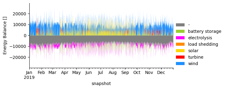
Energy balances plot as time series (in MW):
[6]:
n.statistics.energy_balance.plot.area(linewidth=0, bus_carrier="electricity")
[6]:
(<Figure size 758.25x300 with 1 Axes>,
 <Axes: xlabel='snapshot', ylabel='Energy Balance []'>,
 <seaborn.axisgrid.FacetGrid at 0x79022038d400>)
Find lowest wind capacity within 5% cost slack#
The function n.optimize.optimize_mga takes three main arguments:
The
slackfor the allowed relative cost deviation from the cost-optimum (0.05 corresponds to 5%).A dictionary of weights for defining the new objective function. The first level defines the component (e.g. “Generator”), the second level defines the optimisation variable (e.g.
p_nomfor investment), and the third level defines the component name (e.g. fromn.generators.index).The
sense, noting whether to minimizes (“min”) or maximize (“max”) the new objective.
[7]:
weights = {"Generator": {"p_nom": {"wind": 1}}}
n.optimize.optimize_mga(slack=0.05, weights=weights, sense="min", solver_name="highs")
INFO:linopy.model: Solve problem using Highs solver
INFO:linopy.io:Writing objective.
Writing constraints.: 100%|██████████| 26/26 [00:00<00:00, 84.63it/s]
Writing continuous variables.: 100%|██████████| 11/11 [00:00<00:00, 209.19it/s]
INFO:linopy.io: Writing time: 0.37s
Running HiGHS 1.11.0 (git hash: 364c83a): Copyright (c) 2025 HiGHS under MIT licence terms
LP   linopy-problem-lrn1639l has 64247 rows; 29206 cols; 127070 nonzeros
Coefficient ranges:
  Matrix [2e-04, 2e+05]
  Cost   [1e+00, 1e+00]
  Bound  [0e+00, 0e+00]
  RHS    [5e+03, 8e+09]
Presolving model
33619 rows, 27784 cols, 95020 nonzeros  0s
Dependent equations search running on 8760 equations with time limit of 1000.00s
Dependent equations search removed 0 rows and 0 nonzeros in 0.00s (limit = 1000.00s)
30699 rows, 24864 cols, 89180 nonzeros  0s
Presolve : Reductions: rows 30699(-33548); columns 24864(-4342); elements 89180(-37890)
Solving the presolved LP
Using EKK dual simplex solver - serial
  Iteration        Objective     Infeasibilities num(sum)
          0     0.0000000000e+00 Pr: 2920(1.05973e+08) 0s
      14141     1.8121962939e+04 Pr: 15915(3.26167e+10); Du: 0(1.31772e-05) 5s
INFO:linopy.constants: Optimization successful:
Status: ok
Termination condition: optimal
Solution: 29206 primals, 64247 duals
Objective: 2.13e+04
Solver model: available
Solver message: Optimal
      19422     2.1334327639e+04 Pr: 0(0) 9s
      19422     2.1334327639e+04 Pr: 0(0) 9s
Solving the original LP from the solution after postsolve
Model name          : linopy-problem-lrn1639l
Model status        : Optimal
Simplex   iterations: 19422
Objective value     :  2.1334327639e+04
P-D objective error :  2.3019972191e-15
HiGHS run time      :          8.85
Writing the solution to /tmp/linopy-solve-kcv_wrt2.sol
INFO:pypsa.optimization.optimize:The shadow-prices of the constraints Generator-fix-p-lower, Generator-fix-p-upper, Generator-ext-p-lower, Generator-ext-p-upper, Link-ext-p-lower, Link-ext-p-upper, Store-ext-e-lower, Store-ext-e-upper, StorageUnit-ext-p_dispatch-lower, StorageUnit-ext-p_dispatch-upper, StorageUnit-ext-p_store-lower, StorageUnit-ext-p_store-upper, StorageUnit-ext-state_of_charge-lower, StorageUnit-ext-state_of_charge-upper, StorageUnit-energy_balance, Store-energy_balance, budget were not assigned to the network.
[7]:
('ok', 'optimal')
The breakdown of total system costs shifts from wind towards more solar.
[8]:
tsc = (
    pd.concat([n.statistics.capex(), n.statistics.opex()], axis=1).sum(axis=1).div(1e9)
)
tsc
[8]:
component    carrier
Generator    solar               2.133254
             wind                2.168509
Link         electrolysis        0.539322
             turbine             1.191285
StorageUnit  battery storage     1.402346
Store        hydrogen storage    0.903488
Generator    load shedding       0.143837
dtype: float64
Up to numeric differences, it is 5% more expensive overall:
[9]:
optimal_cost * 1.05
[9]:
np.float64(8.482042459223813)
[10]:
tsc.sum()
[10]:
np.float64(8.48204245921775)
Overall, the wind capacity is cut by roughly a third:
[11]:
n.statistics.optimal_capacity().div(1e3)
[11]:
component    carrier
Generator    load shedding         10.901160
             solar                 41.545979
             wind                  21.334328
Link         electrolysis           2.857854
             turbine               10.235553
StorageUnit  battery storage       22.132377
Store        hydrogen storage    6091.522243
dtype: float64
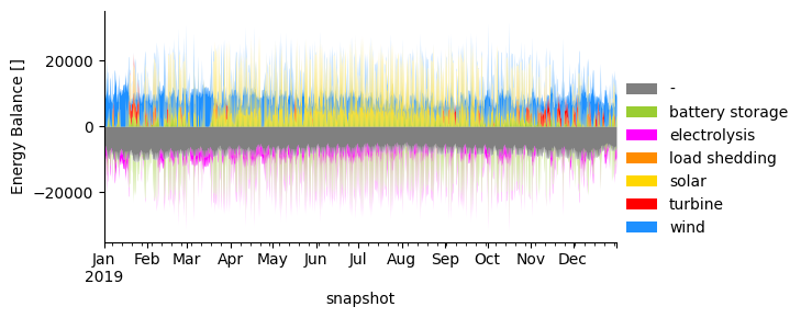
This is also evident in the energy balance:
[12]:
n.statistics.energy_balance(bus_carrier="electricity").sort_values().div(1e6)
[12]:
component    carrier          bus_carrier
Load         -                electricity   -66.266089
Link         electrolysis     electricity   -14.552445
StorageUnit  battery storage  electricity    -1.335461
Generator    load shedding    electricity     0.071919
Link         turbine          electricity     3.709375
Generator    wind             electricity    37.565242
             solar            electricity    40.807460
dtype: float64
And also recognizable in the energy balance time series plots:
[13]:
n.statistics.energy_balance.plot.area(linewidth=0, bus_carrier="electricity")
[13]:
(<Figure size 758.25x300 with 1 Axes>,
 <Axes: xlabel='snapshot', ylabel='Energy Balance []'>,
 <seaborn.axisgrid.FacetGrid at 0x7901d90ca350>)
[ ]: