Note
You can download this example as a Jupyter notebook or start it in interactive mode.
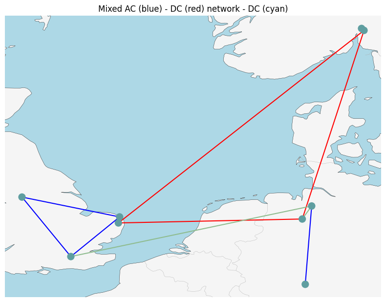
Meshed AC-DC example#
This example has a 3-node AC network coupled via AC-DC converters to a 3-node DC network. There is also a single point-to-point DC using the Link component.
The data files for this example are in the examples folder of the github repository: PyPSA/PyPSA.
[1]:
import matplotlib.pyplot as plt

import pypsa

%matplotlib inline
plt.rc("figure", figsize=(8, 8))
[2]:
network = pypsa.examples.ac_dc_meshed(from_master=True)
WARNING:pypsa.io:Importing network from PyPSA version v0.17.1 while current version is v0.34.0. Read the release notes at https://pypsa.readthedocs.io/en/latest/release_notes.html to prepare your network for import.
INFO:pypsa.io:Imported network ac-dc-meshed.nc has buses, carriers, generators, global_constraints, lines, links, loads
[3]:
# get current type (AC or DC) of the lines from the buses
lines_current_type = network.lines.bus0.map(network.buses.carrier)
lines_current_type
[3]:
Line
0    AC
1    AC
2    DC
3    DC
4    DC
5    AC
6    AC
Name: bus0, dtype: object
[4]:
network.plot(
    line_colors=lines_current_type.map(lambda ct: "r" if ct == "DC" else "b"),
    title="Mixed AC (blue) - DC (red) network - DC (cyan)",
    color_geomap=True,
    jitter=0.3,
)
plt.tight_layout()
/tmp/ipykernel_872/1053005155.py:1: DeprecatedWarning: plot is deprecated. Use `n.plot.map()` as a drop-in replacement instead.
  network.plot(
/home/docs/checkouts/readthedocs.org/user_builds/pypsa/envs/v0.34.0/lib/python3.13/site-packages/pypsa/plot/accessor.py:34: DeprecationWarning: `color_geomap` is deprecated as an argument to `plot`; use `geomap_colors` instead.
  return plot(self.n, *args, **kwargs)
/home/docs/checkouts/readthedocs.org/user_builds/pypsa/envs/v0.34.0/lib/python3.13/site-packages/cartopy/io/__init__.py:241: DownloadWarning: Downloading: https://naturalearth.s3.amazonaws.com/50m_physical/ne_50m_land.zip
  warnings.warn(f'Downloading: {url}', DownloadWarning)
/home/docs/checkouts/readthedocs.org/user_builds/pypsa/envs/v0.34.0/lib/python3.13/site-packages/cartopy/io/__init__.py:241: DownloadWarning: Downloading: https://naturalearth.s3.amazonaws.com/50m_physical/ne_50m_ocean.zip
  warnings.warn(f'Downloading: {url}', DownloadWarning)
/home/docs/checkouts/readthedocs.org/user_builds/pypsa/envs/v0.34.0/lib/python3.13/site-packages/cartopy/io/__init__.py:241: DownloadWarning: Downloading: https://naturalearth.s3.amazonaws.com/50m_cultural/ne_50m_admin_0_boundary_lines_land.zip
  warnings.warn(f'Downloading: {url}', DownloadWarning)
/home/docs/checkouts/readthedocs.org/user_builds/pypsa/envs/v0.34.0/lib/python3.13/site-packages/cartopy/io/__init__.py:241: DownloadWarning: Downloading: https://naturalearth.s3.amazonaws.com/50m_physical/ne_50m_coastline.zip
  warnings.warn(f'Downloading: {url}', DownloadWarning)
[5]:
network.links.loc["Norwich Converter", "p_nom_extendable"] = False
We inspect the topology of the network. Therefore use the function determine_network_topology and inspect the subnetworks in network.sub_networks.
[6]:
network.determine_network_topology()
network.sub_networks["n_branches"] = [
    len(sn.branches()) for sn in network.sub_networks.obj
]
network.sub_networks["n_buses"] = [len(sn.buses()) for sn in network.sub_networks.obj]

network.sub_networks
[6]:
| carrier | slack_bus | obj | n_branches | n_buses | |
|---|---|---|---|---|---|
| SubNetwork | |||||
| 0 | AC | Manchester | <pypsa.networks.SubNetwork object at 0x7bf3344... | 3 | 3 |
| 1 | DC | Norwich DC | <pypsa.networks.SubNetwork object at 0x7bf32ed... | 3 | 3 |
| 2 | AC | Frankfurt | <pypsa.networks.SubNetwork object at 0x7bf32ed... | 1 | 2 |
| 3 | AC | Norway | <pypsa.networks.SubNetwork object at 0x7bf32ed... | 0 | 1 |
The network covers 10 time steps. These are given by the snapshots attribute.
[7]:
network.snapshots
[7]:
DatetimeIndex(['2015-01-01 00:00:00', '2015-01-01 01:00:00',
               '2015-01-01 02:00:00', '2015-01-01 03:00:00',
               '2015-01-01 04:00:00', '2015-01-01 05:00:00',
               '2015-01-01 06:00:00', '2015-01-01 07:00:00',
               '2015-01-01 08:00:00', '2015-01-01 09:00:00'],
              dtype='datetime64[ns]', name='snapshot', freq=None)
There are 6 generators in the network, 3 wind and 3 gas. All are attached to buses:
[8]:
network.generators
[8]:
| bus | control | type | p_nom | p_nom_mod | p_nom_extendable | p_nom_min | p_nom_max | p_min_pu | p_max_pu | ... | min_up_time | min_down_time | up_time_before | down_time_before | ramp_limit_up | ramp_limit_down | ramp_limit_start_up | ramp_limit_shut_down | weight | p_nom_opt | |
|---|---|---|---|---|---|---|---|---|---|---|---|---|---|---|---|---|---|---|---|---|---|
| Generator | |||||||||||||||||||||
| Manchester Wind | Manchester | Slack | 80.0 | 0.0 | True | 100.0 | inf | 0.0 | 1.0 | ... | 0 | 0 | 1 | 0 | NaN | NaN | 1.0 | 1.0 | 1.0 | 0.0 | |
| Manchester Gas | Manchester | PQ | 50000.0 | 0.0 | True | 0.0 | inf | 0.0 | 1.0 | ... | 0 | 0 | 1 | 0 | NaN | NaN | 1.0 | 1.0 | 1.0 | 0.0 | |
| Norway Wind | Norway | Slack | 100.0 | 0.0 | True | 100.0 | inf | 0.0 | 1.0 | ... | 0 | 0 | 1 | 0 | NaN | NaN | 1.0 | 1.0 | 1.0 | 0.0 | |
| Norway Gas | Norway | PQ | 20000.0 | 0.0 | True | 0.0 | inf | 0.0 | 1.0 | ... | 0 | 0 | 1 | 0 | NaN | NaN | 1.0 | 1.0 | 1.0 | 0.0 | |
| Frankfurt Wind | Frankfurt | Slack | 110.0 | 0.0 | True | 100.0 | inf | 0.0 | 1.0 | ... | 0 | 0 | 1 | 0 | NaN | NaN | 1.0 | 1.0 | 1.0 | 0.0 | |
| Frankfurt Gas | Frankfurt | PQ | 80000.0 | 0.0 | True | 0.0 | inf | 0.0 | 1.0 | ... | 0 | 0 | 1 | 0 | NaN | NaN | 1.0 | 1.0 | 1.0 | 0.0 |
6 rows × 37 columns
We see that the generators have different capital and marginal costs. All of them have a p_nom_extendable set to True, meaning that capacities can be extended in the optimization.
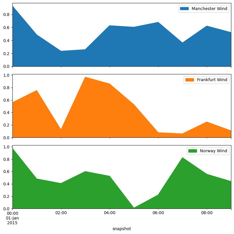
The wind generators have a per unit limit for each time step, given by the weather potentials at the site.
[9]:
network.generators_t.p_max_pu.plot.area(subplots=True)
plt.tight_layout()
Alright now we know how the network looks like, where the generators and lines are. Now, let’s perform a optimization of the operation and capacities.
[10]:
network.optimize();
WARNING:pypsa.consistency:The following lines have zero x, which could break the linear load flow:
Index(['2', '3', '4'], dtype='object', name='Line')
WARNING:pypsa.consistency:The following lines have zero r, which could break the linear load flow:
Index(['0', '1', '5', '6'], dtype='object', name='Line')
INFO:linopy.model: Solve problem using Highs solver
INFO:linopy.io: Writing time: 0.06s
INFO:linopy.constants: Optimization successful:
Status: ok
Termination condition: optimal
Solution: 187 primals, 467 duals
Objective: -3.47e+06
Solver model: available
Solver message: optimal

INFO:pypsa.optimization.optimize:The shadow-prices of the constraints Generator-ext-p-lower, Generator-ext-p-upper, Line-ext-s-lower, Line-ext-s-upper, Link-fix-p-lower, Link-fix-p-upper, Link-ext-p-lower, Link-ext-p-upper, Kirchhoff-Voltage-Law were not assigned to the network.
Running HiGHS 1.10.0 (git hash: fd86653): Copyright (c) 2025 HiGHS under MIT licence terms
LP   linopy-problem-f98zrkc7 has 467 rows; 187 cols; 986 nonzeros
Coefficient ranges:
  Matrix [1e-02, 1e+00]
  Cost   [9e-03, 3e+03]
  Bound  [2e+07, 2e+07]
  RHS    [9e-01, 1e+03]
Presolving model
371 rows, 186 cols, 890 nonzeros  0s
283 rows, 98 cols, 948 nonzeros  0s
Dependent equations search running on 22 equations with time limit of 1000.00s
Dependent equations search removed 0 rows and 0 nonzeros in 0.00s (limit = 1000.00s)
283 rows, 98 cols, 948 nonzeros  0s
Presolve : Reductions: rows 283(-184); columns 98(-89); elements 948(-38)
Solving the presolved LP
Using EKK dual simplex solver - serial
  Iteration        Objective     Infeasibilities num(sum)
          0    -2.1204300613e+07 Pr: 110(90228.6); Du: 0(1.47603e-11) 0s
         96    -3.4740941308e+06 Pr: 0(0); Du: 0(1.57124e-13) 0s
Solving the original LP from the solution after postsolve
Model name          : linopy-problem-f98zrkc7
Model status        : Optimal
Simplex   iterations: 96
Objective value     : -3.4740941308e+06
Relative P-D gap    :  2.6807637892e-15
HiGHS run time      :          0.00
Writing the solution to /tmp/linopy-solve-gznuo_4r.sol
The objective is given by:
[11]:
network.objective
[11]:
-3474094.1308449395
Why is this number negative? It considers the starting point of the optimization, thus the existent capacities given by network.generators.p_nom are taken into account.
The real system cost are given by
[12]:
network.objective + network.objective_constant
[12]:
np.float64(18440973.387434203)
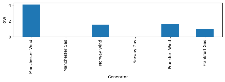
The optimal capacities are given by p_nom_opt for generators, links and storages and s_nom_opt for lines.
Let’s look how the optimal capacities for the generators look like.
[13]:
network.generators.p_nom_opt.div(1e3).plot.bar(ylabel="GW", figsize=(8, 3))
plt.tight_layout()
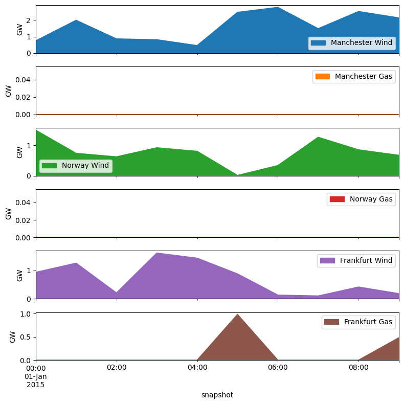
Their production is again given as a time-series in network.generators_t.
[14]:
network.generators_t.p.div(1e3).plot.area(subplots=True, ylabel="GW")
plt.tight_layout()
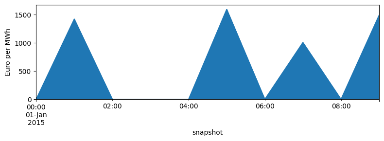
What are the Locational Marginal Prices in the network. From the optimization these are given for each bus and snapshot.
[15]:
network.buses_t.marginal_price.mean(1).plot.area(figsize=(8, 3), ylabel="Euro per MWh")
plt.tight_layout()
We can inspect further quantities as the active power of AC-DC converters and HVDC link.
[16]:
network.links_t.p0
[16]:
| Link | Norwich Converter | Norway Converter | Bremen Converter | DC link |
|---|---|---|---|---|
| snapshot | ||||
| 2015-01-01 00:00:00 | -250.841318 | 674.584826 | -423.743508 | -317.997991 |
| 2015-01-01 01:00:00 | 315.068611 | -116.727192 | -198.341419 | -317.997991 |
| 2015-01-01 02:00:00 | 350.761618 | 581.970687 | -932.732306 | -317.997991 |
| 2015-01-01 03:00:00 | -85.772148 | 272.557949 | -186.785801 | -317.997991 |
| 2015-01-01 04:00:00 | 317.366721 | -79.749487 | -237.617234 | -317.997991 |
| 2015-01-01 05:00:00 | 386.747627 | -494.197717 | 107.450090 | -317.997991 |
| 2015-01-01 06:00:00 | 900.000000 | -257.520720 | -642.479280 | 317.997991 |
| 2015-01-01 07:00:00 | 123.677319 | 971.918845 | -1095.596165 | -86.858742 |
| 2015-01-01 08:00:00 | 244.715828 | 850.880337 | -1095.596165 | 317.997991 |
| 2015-01-01 09:00:00 | 820.022865 | -86.851803 | -733.171062 | -83.684817 |
[17]:
network.lines_t.p0
[17]:
| Line | 0 | 1 | 2 | 3 | 4 | 5 | 6 |
|---|---|---|---|---|---|---|---|
| snapshot | |||||||
| 2015-01-01 00:00:00 | 79.474931 | -38.105568 | -52.967153 | -303.808471 | 370.776355 | -202.726815 | -534.340860 |
| 2015-01-01 01:00:00 | -449.464018 | 787.037310 | -211.273022 | 103.795589 | -12.931603 | 209.362553 | -823.210906 |
| 2015-01-01 02:00:00 | -181.265945 | 520.561348 | -505.913540 | -155.151921 | 426.818766 | -248.676623 | 173.898185 |
| 2015-01-01 03:00:00 | -45.472529 | 234.470017 | -34.040733 | -119.812880 | 152.745069 | -232.717375 | -743.788495 |
| 2015-01-01 04:00:00 | -73.207796 | 295.420961 | -227.198461 | 90.168260 | 10.418773 | -240.105618 | -883.817538 |
| 2015-01-01 05:00:00 | -594.500052 | 1198.082901 | -125.903894 | 260.843733 | -233.353984 | 19.359009 | -1030.848768 |
| 2015-01-01 06:00:00 | -661.294714 | 1378.422245 | -632.371427 | 267.628573 | 10.107853 | -53.448436 | 319.386680 |
| 2015-01-01 07:00:00 | -383.768641 | 540.906725 | -469.925715 | -346.248396 | 625.670450 | 393.715939 | 600.728881 |
| 2015-01-01 08:00:00 | -778.280943 | 1444.069207 | -522.116240 | -277.400413 | 573.479924 | 229.294311 | 501.346379 |
| 2015-01-01 09:00:00 | -465.576406 | 899.565461 | -632.371427 | 187.651438 | 100.799635 | 78.617762 | -248.566847 |
…or the active power injection per bus.
[18]:
network.buses_t.p
[18]:
| Bus | London | Norwich | Norwich DC | Manchester | Bremen | Bremen DC | Frankfurt | Norway | Norway DC |
|---|---|---|---|---|---|---|---|---|---|
| snapshot | |||||||||
| 2015-01-01 00:00:00 | 282.201747 | -164.621247 | -250.841318 | -117.580500 | -534.340860 | -423.743508 | 534.340860 | 0.000000e+00 | 674.584826 |
| 2015-01-01 01:00:00 | -658.826571 | -577.674757 | 315.068611 | 1236.501328 | -823.210906 | -198.341419 | 823.210906 | 2.000888e-10 | -116.727192 |
| 2015-01-01 02:00:00 | 67.410679 | -769.237972 | 350.761618 | 701.827293 | 173.898185 | -932.732306 | -173.898185 | 0.000000e+00 | 581.970687 |
| 2015-01-01 03:00:00 | 187.244846 | -467.187392 | -85.772148 | 279.942546 | -743.788495 | -186.785801 | 743.788495 | -1.000444e-10 | 272.557949 |
| 2015-01-01 04:00:00 | 166.897822 | -535.526579 | 317.366721 | 368.628757 | -883.817538 | -237.617234 | 883.817538 | 3.999503e-10 | -79.749487 |
| 2015-01-01 05:00:00 | -613.859061 | -1178.723892 | 386.747627 | 1792.582954 | -1030.848768 | 107.450090 | 1030.848768 | 3.999503e-10 | -494.197717 |
| 2015-01-01 06:00:00 | -607.846278 | -1431.870681 | 900.000000 | 2039.716959 | 319.386680 | -642.479280 | -319.386680 | 2.999059e-10 | -257.520720 |
| 2015-01-01 07:00:00 | -777.484580 | -147.190786 | 123.677319 | 924.675366 | 600.728881 | -1095.596165 | -600.728881 | -3.999503e-10 | 971.918845 |
| 2015-01-01 08:00:00 | -1007.575254 | -1214.774896 | 244.715828 | 2222.350150 | 501.346379 | -1095.596165 | -501.346379 | 0.000000e+00 | 850.880337 |
| 2015-01-01 09:00:00 | -544.194169 | -820.947699 | 820.022865 | 1365.141868 | -248.566847 | -733.171062 | 248.566847 | 2.000888e-10 | -86.851803 |