Note

You can download this example as a Jupyter notebook or start it in interactive mode.

Redispatch Example with SciGRID network#

In this example, we compare a 2-stage market with an initial market clearing in two bidding zones with flow-based market coupling and a subsequent redispatch market (incl. curtailment) to an idealised nodal pricing scheme.

[1]:

import cartopy.crs as ccrs
import matplotlib.pyplot as plt

import pypsa
from pypsa.descriptors import get_switchable_as_dense as as_dense

Load example network#

[2]:

o = pypsa.examples.scigrid_de(from_master=True)
o.lines.s_max_pu = 0.7
o.lines.loc[["316", "527", "602"], "s_nom"] = 1715
o.set_snapshots([o.snapshots[12]])

WARNING:pypsa.io:Importing network from PyPSA version v0.17.1 while current version is v0.33.1. Read the release notes at https://pypsa.readthedocs.io/en/latest/release_notes.html to prepare your network for import.
INFO:pypsa.io:Imported network scigrid-de.nc has buses, generators, lines, loads, storage_units, transformers

[3]:

n = o.copy()  # for redispatch model
m = o.copy()  # for market model

[4]:

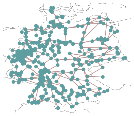
o.plot();

/home/docs/checkouts/readthedocs.org/user_builds/pypsa/envs/v0.33.1/lib/python3.13/site-packages/cartopy/mpl/feature_artist.py:144: UserWarning: facecolor will have no effect as it has been defined as "never".
  warnings.warn('facecolor will have no effect as it has been '

../_images/examples_scigrid-redispatch_5_1.png

Solve original nodal market model `o`#

First, let us solve a nodal market using the original model o:

[5]:

o.optimize()

WARNING:pypsa.consistency:The following transformers have zero r, which could break the linear load flow:
Index(['2', '5', '10', '12', '13', '15', '18', '20', '22', '24', '26', '30',
       '32', '37', '42', '46', '52', '56', '61', '68', '69', '74', '78', '86',
       '87', '94', '95', '96', '99', '100', '104', '105', '106', '107', '117',
       '120', '123', '124', '125', '128', '129', '138', '143', '156', '157',
       '159', '160', '165', '184', '191', '195', '201', '220', '231', '232',
       '233', '236', '247', '248', '250', '251', '252', '261', '263', '264',
       '267', '272', '279', '281', '282', '292', '303', '307', '308', '312',
       '315', '317', '322', '332', '334', '336', '338', '351', '353', '360',
       '362', '382', '384', '385', '391', '403', '404', '413', '421', '450',
       '458'],
      dtype='object', name='Transformer')
INFO:linopy.model: Solve problem using Highs solver
INFO:linopy.io: Writing time: 0.16s
INFO:linopy.constants: Optimization successful:
Status: ok
Termination condition: optimal
Solution: 2485 primals, 5957 duals
Objective: 3.01e+05
Solver model: available
Solver message: optimal

Running HiGHS 1.9.0 (git hash: fa40bdf): Copyright (c) 2024 HiGHS under MIT licence terms
Coefficient ranges:
  Matrix [1e-02, 2e+02]
  Cost   [3e+00, 1e+02]
  Bound  [0e+00, 0e+00]
  RHS    [4e-10, 6e+03]
Presolving model
817 rows, 2282 cols, 5150 nonzeros  0s
559 rows, 2017 cols, 4767 nonzeros  0s
543 rows, 1362 cols, 4040 nonzeros  0s
524 rows, 1338 cols, 4071 nonzeros  0s
Presolve : Reductions: rows 524(-5433); columns 1338(-1147); elements 4071(-6780)
Solving the presolved LP
Using EKK dual simplex solver - serial
  Iteration        Objective     Infeasibilities num(sum)
          0    -2.3328331372e-01 Pr: 486(3.28207e+06) 0s
        641     3.0120938233e+05 Pr: 0(0) 0s
Solving the original LP from the solution after postsolve
Model name          : linopy-problem-omkzpgcv
Model status        : Optimal
Simplex   iterations: 641
Objective value     :  3.0120938233e+05
Relative P-D gap    :  9.6623253340e-16
HiGHS run time      :          0.06
Writing the solution to /tmp/linopy-solve-21mb4qht.sol

INFO:pypsa.optimization.optimize:The shadow-prices of the constraints Generator-fix-p-lower, Generator-fix-p-upper, Line-fix-s-lower, Line-fix-s-upper, Transformer-fix-s-lower, Transformer-fix-s-upper, StorageUnit-fix-p_dispatch-lower, StorageUnit-fix-p_dispatch-upper, StorageUnit-fix-p_store-lower, StorageUnit-fix-p_store-upper, StorageUnit-fix-state_of_charge-lower, StorageUnit-fix-state_of_charge-upper, Kirchhoff-Voltage-Law, StorageUnit-energy_balance were not assigned to the network.

[5]:

('ok', 'optimal')

Costs are 301 k€.

Build market model `m` with two bidding zones#

For this example, we split the German transmission network into two market zones at latitude 51 degrees.

You can build any other market zones by providing an alternative mapping from bus to zone.

[6]:

zones = (n.buses.y > 51).map(lambda x: "North" if x else "South")

Next, we assign this mapping to the market model m.

We re-assign the buses of all generators and loads, and remove all transmission lines within each bidding zone.

Here, we assume that the bidding zones are coupled through the transmission lines that connect them.

[7]:

for c in m.iterate_components(m.one_port_components):
    c.static.bus = c.static.bus.map(zones)

for c in m.iterate_components(m.branch_components):
    c.static.bus0 = c.static.bus0.map(zones)
    c.static.bus1 = c.static.bus1.map(zones)
    internal = c.static.bus0 == c.static.bus1
    m.remove(c.name, c.static.loc[internal].index)

m.remove("Bus", m.buses.index)
m.add("Bus", ["North", "South"]);

Now, we can solve the coupled market with two bidding zones.

[8]:

m.optimize()

INFO:linopy.model: Solve problem using Highs solver
INFO:linopy.io: Writing time: 0.11s
INFO:linopy.constants: Optimization successful:
Status: ok
Termination condition: optimal
Solution: 1561 primals, 3185 duals
Objective: 2.14e+05
Solver model: available
Solver message: optimal

INFO:pypsa.optimization.optimize:The shadow-prices of the constraints Generator-fix-p-lower, Generator-fix-p-upper, Line-fix-s-lower, Line-fix-s-upper, StorageUnit-fix-p_dispatch-lower, StorageUnit-fix-p_dispatch-upper, StorageUnit-fix-p_store-lower, StorageUnit-fix-p_store-upper, StorageUnit-fix-state_of_charge-lower, StorageUnit-fix-state_of_charge-upper, Kirchhoff-Voltage-Law, StorageUnit-energy_balance were not assigned to the network.

Running HiGHS 1.9.0 (git hash: fa40bdf): Copyright (c) 2024 HiGHS under MIT licence terms
Coefficient ranges:
  Matrix [9e-01, 3e+06]
  Cost   [3e+00, 1e+02]
  Bound  [0e+00, 0e+00]
  RHS    [4e-10, 3e+04]
Presolving model
40 rows, 1510 cols, 1587 nonzeros  0s
40 rows, 135 cols, 212 nonzeros  0s
40 rows, 135 cols, 212 nonzeros  0s
Presolve : Reductions: rows 40(-3145); columns 135(-1426); elements 212(-4617)
Solving the presolved LP
Using EKK dual simplex solver - serial
  Iteration        Objective     Infeasibilities num(sum)
          0    -4.3458587374e-04 Pr: 2(51830.2) 0s
         42     2.1398868596e+05 Pr: 0(0) 0s
Solving the original LP from the solution after postsolve
Model name          : linopy-problem-7vh_9b95
Model status        : Optimal
Simplex   iterations: 42
Objective value     :  2.1398868596e+05
Relative P-D gap    :  6.2562943224e-15
HiGHS run time      :          0.01
Writing the solution to /tmp/linopy-solve-c29dtwmv.sol

[8]:

('ok', 'optimal')

Costs are 214 k€, which is much lower than the 301 k€ of the nodal market.

This is because network restrictions apart from the North/South division are not taken into account yet.

We can look at the market clearing prices of each zone:

[9]:

m.buses_t.marginal_price

[9]:

Bus	North	South
snapshot
2011-01-01 12:00:00	8.0	25.0

Build redispatch model `n`#

Next, based on the market outcome with two bidding zones m, we build a secondary redispatch market n that rectifies transmission constraints through curtailment and ramping up/down thermal generators.

First, we fix the dispatch of generators to the results from the market simulation. (For simplicity, this example disregards storage units.)

[10]:

p = m.generators_t.p / m.generators.p_nom
n.generators_t.p_min_pu = p
n.generators_t.p_max_pu = p

Then, we add generators bidding into redispatch market using the following assumptions:

All generators can reduce their dispatch to zero. This includes also curtailment of renewables.
All generators can increase their dispatch to their available/nominal capacity.
No changes to the marginal costs, i.e. reducing dispatch lowers costs.

With these settings, the 2-stage market should result in the same cost as the nodal market.

[11]:

g_up = n.generators.copy()
g_down = n.generators.copy()

g_up.index = g_up.index.map(lambda x: x + " ramp up")
g_down.index = g_down.index.map(lambda x: x + " ramp down")

up = (
    as_dense(m, "Generator", "p_max_pu") * m.generators.p_nom - m.generators_t.p
).clip(0) / m.generators.p_nom
down = -m.generators_t.p / m.generators.p_nom

up.columns = up.columns.map(lambda x: x + " ramp up")
down.columns = down.columns.map(lambda x: x + " ramp down")

n.add("Generator", g_up.index, p_max_pu=up, **g_up.drop("p_max_pu", axis=1))

n.add(
    "Generator",
    g_down.index,
    p_min_pu=down,
    p_max_pu=0,
    **g_down.drop(["p_max_pu", "p_min_pu"], axis=1),
);

Now, let’s solve the redispatch market:

[12]:

n.optimize()

WARNING:pypsa.consistency:The following transformers have zero r, which could break the linear load flow:
Index(['2', '5', '10', '12', '13', '15', '18', '20', '22', '24', '26', '30',
       '32', '37', '42', '46', '52', '56', '61', '68', '69', '74', '78', '86',
       '87', '94', '95', '96', '99', '100', '104', '105', '106', '107', '117',
       '120', '123', '124', '125', '128', '129', '138', '143', '156', '157',
       '159', '160', '165', '184', '191', '195', '201', '220', '231', '232',
       '233', '236', '247', '248', '250', '251', '252', '261', '263', '264',
       '267', '272', '279', '281', '282', '292', '303', '307', '308', '312',
       '315', '317', '322', '332', '334', '336', '338', '351', '353', '360',
       '362', '382', '384', '385', '391', '403', '404', '413', '421', '450',
       '458'],
      dtype='object', name='Transformer')
INFO:linopy.model: Solve problem using Highs solver
INFO:linopy.io: Writing time: 0.22s
INFO:linopy.constants: Optimization successful:
Status: ok
Termination condition: optimal
Solution: 5331 primals, 11649 duals
Objective: 3.01e+05
Solver model: available
Solver message: optimal

Running HiGHS 1.9.0 (git hash: fa40bdf): Copyright (c) 2024 HiGHS under MIT licence terms
Coefficient ranges:
  Matrix [1e-02, 2e+02]
  Cost   [3e+00, 1e+02]
  Bound  [0e+00, 0e+00]
  RHS    [2e-19, 6e+03]
Presolving model
817 rows, 2285 cols, 5153 nonzeros  0s
560 rows, 2020 cols, 4774 nonzeros  0s
544 rows, 1363 cols, 4045 nonzeros  0s
528 rows, 1342 cols, 4107 nonzeros  0s
Presolve : Reductions: rows 528(-11121); columns 1342(-3989); elements 4107(-15282)
Solving the presolved LP
Using EKK dual simplex solver - serial
  Iteration        Objective     Infeasibilities num(sum)
          0     0.0000000000e+00 Ph1: 0(0) 0s
        633     3.0120938233e+05 Pr: 0(0); Du: 0(2.57572e-14) 0s
Solving the original LP from the solution after postsolve
Model name          : linopy-problem-na6waldl
Model status        : Optimal
Simplex   iterations: 633
Objective value     :  3.0120938232e+05
Relative P-D gap    :  5.6041486937e-15
HiGHS run time      :          0.07
Writing the solution to /tmp/linopy-solve-ycvroxf4.sol

INFO:pypsa.optimization.optimize:The shadow-prices of the constraints Generator-fix-p-lower, Generator-fix-p-upper, Line-fix-s-lower, Line-fix-s-upper, Transformer-fix-s-lower, Transformer-fix-s-upper, StorageUnit-fix-p_dispatch-lower, StorageUnit-fix-p_dispatch-upper, StorageUnit-fix-p_store-lower, StorageUnit-fix-p_store-upper, StorageUnit-fix-state_of_charge-lower, StorageUnit-fix-state_of_charge-upper, Kirchhoff-Voltage-Law, StorageUnit-energy_balance were not assigned to the network.

[12]:

('ok', 'optimal')

And, as expected, the costs are the same as for the nodal market: 301 k€.

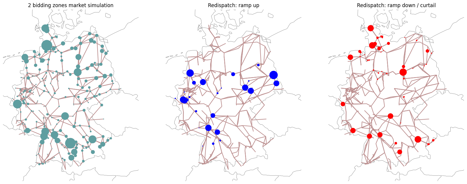
Now, we can plot both the market results of the 2 bidding zone market and the redispatch results:

[13]:

fig, axs = plt.subplots(
    1, 3, figsize=(20, 10), subplot_kw={"projection": ccrs.AlbersEqualArea()}
)

market = (
    n.generators_t.p[m.generators.index]
    .T.squeeze()
    .groupby(n.generators.bus)
    .sum()
    .div(2e4)
)
n.plot(ax=axs[0], bus_sizes=market, title="2 bidding zones market simulation")

redispatch_up = (
    n.generators_t.p.filter(like="ramp up")
    .T.squeeze()
    .groupby(n.generators.bus)
    .sum()
    .div(2e4)
)
n.plot(
    ax=axs[1], bus_sizes=redispatch_up, bus_colors="blue", title="Redispatch: ramp up"
)

redispatch_down = (
    n.generators_t.p.filter(like="ramp down")
    .T.squeeze()
    .groupby(n.generators.bus)
    .sum()
    .div(-2e4)
)
n.plot(
    ax=axs[2],
    bus_sizes=redispatch_down,
    bus_colors="red",
    title="Redispatch: ramp down / curtail",
);

/home/docs/checkouts/readthedocs.org/user_builds/pypsa/envs/v0.33.1/lib/python3.13/site-packages/cartopy/mpl/feature_artist.py:144: UserWarning: facecolor will have no effect as it has been defined as "never".
  warnings.warn('facecolor will have no effect as it has been '
/home/docs/checkouts/readthedocs.org/user_builds/pypsa/envs/v0.33.1/lib/python3.13/site-packages/cartopy/mpl/feature_artist.py:144: UserWarning: facecolor will have no effect as it has been defined as "never".
  warnings.warn('facecolor will have no effect as it has been '
/home/docs/checkouts/readthedocs.org/user_builds/pypsa/envs/v0.33.1/lib/python3.13/site-packages/cartopy/mpl/feature_artist.py:144: UserWarning: facecolor will have no effect as it has been defined as "never".
  warnings.warn('facecolor will have no effect as it has been '

../_images/examples_scigrid-redispatch_29_1.png

We can also read out the final dispatch of each generator:

[14]:

grouper = n.generators.index.str.split(" ramp", expand=True).get_level_values(0)

n.generators_t.p.groupby(grouper, axis=1).sum().squeeze()

/tmp/ipykernel_6398/2204001103.py:3: FutureWarning: DataFrame.groupby with axis=1 is deprecated. Do `frame.T.groupby(...)` without axis instead.
  n.generators_t.p.groupby(grouper, axis=1).sum().squeeze()

[14]:

1 Gas                     0.000000
1 Hard Coal               0.000000
1 Solar                  11.326192
1 Wind Onshore            1.754382
100_220kV Solar          14.913326
                           ...
98 Wind Onshore          71.451646
99_220kV Gas              0.000000
99_220kV Hard Coal        0.000000
99_220kV Solar            8.246606
99_220kV Wind Onshore     3.432939
Name: 2011-01-01 12:00:00, Length: 1423, dtype: float64

Changing bidding strategies in redispatch market#

We can also formulate other bidding strategies or compensation mechanisms for the redispatch market.

For example, that ramping up a generator is twice as expensive.

[15]:

n.generators.loc[n.generators.index.str.contains("ramp up"), "marginal_cost"] *= 2

Or that generators need to be compensated for curtailing them or ramping them down at 50% of their marginal cost.

[16]:

n.generators.loc[n.generators.index.str.contains("ramp down"), "marginal_cost"] *= -0.5

In this way, the outcome should be more expensive than the ideal nodal market:

[17]:

n.optimize()

WARNING:pypsa.consistency:The following transformers have zero r, which could break the linear load flow:
Index(['2', '5', '10', '12', '13', '15', '18', '20', '22', '24', '26', '30',
       '32', '37', '42', '46', '52', '56', '61', '68', '69', '74', '78', '86',
       '87', '94', '95', '96', '99', '100', '104', '105', '106', '107', '117',
       '120', '123', '124', '125', '128', '129', '138', '143', '156', '157',
       '159', '160', '165', '184', '191', '195', '201', '220', '231', '232',
       '233', '236', '247', '248', '250', '251', '252', '261', '263', '264',
       '267', '272', '279', '281', '282', '292', '303', '307', '308', '312',
       '315', '317', '322', '332', '334', '336', '338', '351', '353', '360',
       '362', '382', '384', '385', '391', '403', '404', '413', '421', '450',
       '458'],
      dtype='object', name='Transformer')
INFO:linopy.model: Solve problem using Highs solver
INFO:linopy.io: Writing time: 0.22s
INFO:linopy.constants: Optimization successful:
Status: ok
Termination condition: optimal
Solution: 5331 primals, 11649 duals
Objective: 4.99e+05
Solver model: available
Solver message: optimal

Running HiGHS 1.9.0 (git hash: fa40bdf): Copyright (c) 2024 HiGHS under MIT licence terms
Coefficient ranges:
  Matrix [1e-02, 2e+02]
  Cost   [2e+00, 2e+02]
  Bound  [0e+00, 0e+00]
  RHS    [2e-19, 6e+03]
Presolving model
817 rows, 2277 cols, 5145 nonzeros  0s
558 rows, 2004 cols, 4756 nonzeros  0s
541 rows, 1355 cols, 4034 nonzeros  0s
522 rows, 1331 cols, 4065 nonzeros  0s
Presolve : Reductions: rows 522(-11127); columns 1331(-4000); elements 4065(-15324)
Solving the presolved LP
Using EKK dual simplex solver - serial
  Iteration        Objective     Infeasibilities num(sum)
          0     0.0000000000e+00 Ph1: 0(0) 0s
        659     4.9929741194e+05 Pr: 0(0); Du: 0(1.77636e-14) 0s
Solving the original LP from the solution after postsolve
Model name          : linopy-problem-f7y9tmah
Model status        : Optimal
Simplex   iterations: 659
Objective value     :  4.9929741194e+05
Relative P-D gap    :  1.3406600645e-14
HiGHS run time      :          0.07
Writing the solution to /tmp/linopy-solve-mtdf0443.sol

INFO:pypsa.optimization.optimize:The shadow-prices of the constraints Generator-fix-p-lower, Generator-fix-p-upper, Line-fix-s-lower, Line-fix-s-upper, Transformer-fix-s-lower, Transformer-fix-s-upper, StorageUnit-fix-p_dispatch-lower, StorageUnit-fix-p_dispatch-upper, StorageUnit-fix-p_store-lower, StorageUnit-fix-p_store-upper, StorageUnit-fix-state_of_charge-lower, StorageUnit-fix-state_of_charge-upper, Kirchhoff-Voltage-Law, StorageUnit-energy_balance were not assigned to the network.

[17]:

('ok', 'optimal')

Costs are now 502 k€ compared to 301 k€.

Redispatch Example with SciGRID network

Contents

Redispatch Example with SciGRID network#

Load example network#

Solve original nodal market model o#

Build market model m with two bidding zones#

Build redispatch model n#

Changing bidding strategies in redispatch market#

Solve original nodal market model `o`#

Build market model `m` with two bidding zones#

Build redispatch model `n`#