Note
You can download this example as a Jupyter notebook or start it in interactive mode.
Screening curve analysis#
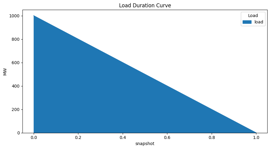
Compute the long-term equilibrium power plant investment for a given load duration curve (1000-1000z for z \(\in\) [0,1]) and a given set of generator investment options.
[1]:
import matplotlib.pyplot as plt
import numpy as np
import pandas as pd

import pypsa
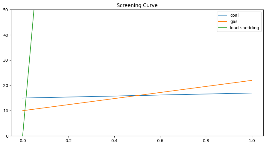
Generator marginal (m) and capital (c) costs in EUR/MWh - numbers chosen for simple answer.
[2]:
generators = {
    "coal": {"m": 2, "c": 15},
    "gas": {"m": 12, "c": 10},
    "load-shedding": {"m": 1012, "c": 0},
}
The screening curve intersections are at 0.01 and 0.5.
[3]:
x = np.linspace(0, 1, 101)
df = pd.DataFrame(
    {key: pd.Series(item["c"] + x * item["m"], x) for key, item in generators.items()}
)
df.plot(ylim=[0, 50], title="Screening Curve", figsize=(9, 5))
plt.tight_layout()
[4]:
n = pypsa.Network()

num_snapshots = 1001
n.snapshots = np.linspace(0, 1, num_snapshots)
n.snapshot_weightings = n.snapshot_weightings / num_snapshots

n.add("Bus", name="bus")

n.add("Load", name="load", bus="bus", p_set=1000 - 1000 * n.snapshots.values)

for gen in generators:
    n.add(
        "Generator",
        name=gen,
        bus="bus",
        p_nom_extendable=True,
        marginal_cost=float(generators[gen]["m"]),
        capital_cost=float(generators[gen]["c"]),
    )
[5]:
n.loads_t.p_set.plot.area(title="Load Duration Curve", figsize=(9, 5), ylabel="MW")
plt.tight_layout()
[6]:
n.optimize()
n.objective
WARNING:pypsa.consistency:The following buses have carriers which are not defined:
Index(['bus'], dtype='object', name='Bus')
WARNING:pypsa.consistency:The following buses have carriers which are not defined:
Index(['bus'], dtype='object', name='Bus')
INFO:linopy.model: Solve problem using Highs solver
INFO:linopy.io: Writing time: 0.08s
INFO:linopy.solvers:Log file at /tmp/highs.log
INFO:linopy.constants: Optimization successful:
Status: ok
Termination condition: optimal
Solution: 3006 primals, 7010 duals
Objective: 1.47e+04
Solver model: available
Solver message: optimal

INFO:pypsa.optimization.optimize:The shadow-prices of the constraints Generator-ext-p-lower, Generator-ext-p-upper were not assigned to the network.
Running HiGHS 1.7.2 (git hash: 184e327): Copyright (c) 2024 HiGHS under MIT licence terms
Coefficient ranges:
  Matrix [1e+00, 1e+00]
  Cost   [2e-03, 2e+01]
  Bound  [0e+00, 0e+00]
  RHS    [1e+00, 1e+03]
Presolving model
3000 rows, 3002 cols, 7000 nonzeros  0s
3000 rows, 3002 cols, 7000 nonzeros  0s
Presolve : Reductions: rows 3000(-4010); columns 3002(-4); elements 7000(-5015)
Solving the presolved LP
Using EKK dual simplex solver - serial
  Iteration        Objective     Infeasibilities num(sum)
          0     0.0000000000e+00 Pr: 1000(500500) 0s
       1512     1.4706193806e+04 Pr: 0(0) 0s
Solving the original LP from the solution after postsolve
Model   status      : Optimal
Simplex   iterations: 1512
Objective value     :  1.4706193806e+04
HiGHS run time      :          0.02
Writing the solution to /tmp/linopy-solve-vmmce1sp.sol
[6]:
14706.193806191455
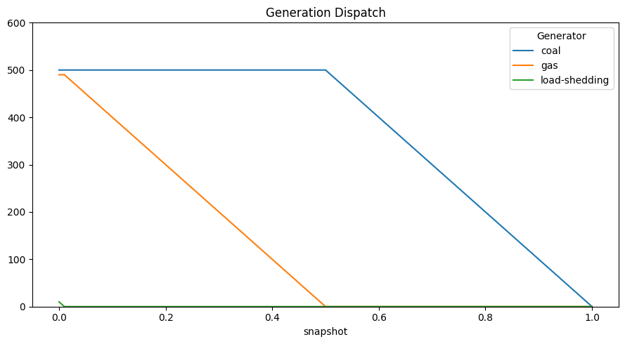
The capacity is set by total electricity required.
NB: No load shedding since all prices are below 10 000.
[7]:
n.generators.p_nom_opt.round(2)
[7]:
Generator
coal             500.0
gas              490.0
load-shedding     10.0
Name: p_nom_opt, dtype: float64
[8]:
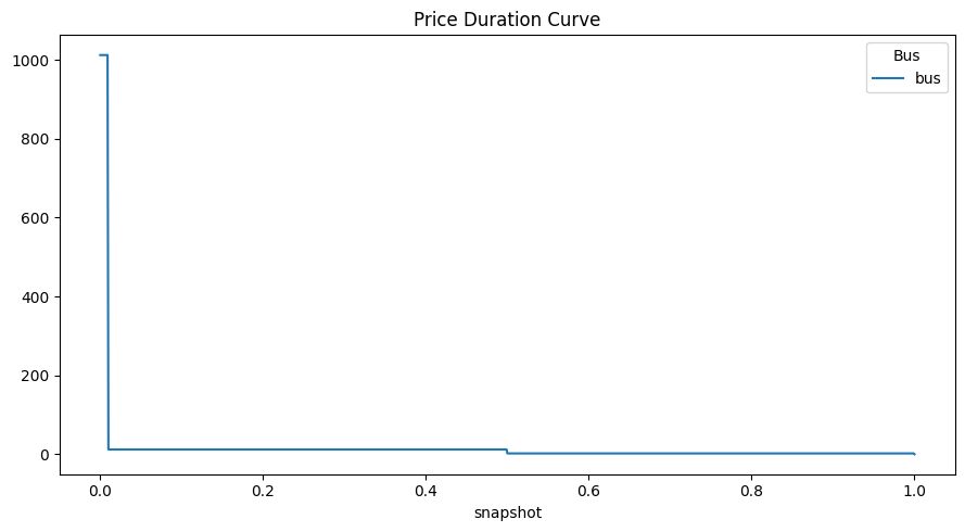
n.buses_t.marginal_price.plot(title="Price Duration Curve", figsize=(9, 4))
plt.tight_layout()
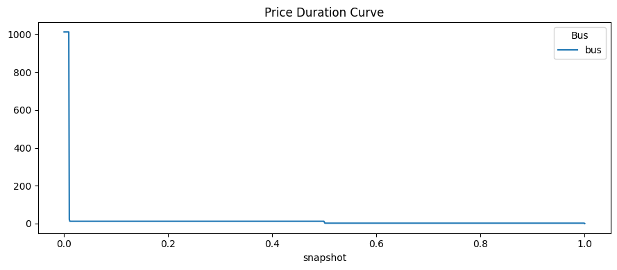
The prices correspond either to VOLL (1012) for first 0.01 or the marginal costs (12 for 0.49 and 2 for 0.5)
Except for (infinitesimally small) points at the screening curve intersections, which correspond to changing the load duration near the intersection, so that capacity changes. This explains 7 = (12+10 - 15) (replacing coal with gas) and 22 = (12+10) (replacing load-shedding with gas).
Note: What remains unclear is what is causing :nbsphinx-math:`l `= 0… it should be 2.
[9]:
n.buses_t.marginal_price.round(2).sum(axis=1).value_counts()
[9]:
2.0       499
12.0      489
1012.0     10
22.0        1
7.0         1
0.0         1
Name: count, dtype: int64
[10]:
n.generators_t.p.plot(ylim=[0, 600], title="Generation Dispatch", figsize=(9, 5))
plt.tight_layout()
Demonstrate zero-profit condition.
The total cost is given by
[11]:
(
    n.generators.p_nom_opt * n.generators.capital_cost
    + n.generators_t.p.multiply(n.snapshot_weightings.generators, axis=0).sum()
    * n.generators.marginal_cost
)
[11]:
Generator
coal             8249.750250
gas              6400.839161
load-shedding      55.604396
dtype: float64
The total revenue by
[12]:
(
    n.generators_t.p.multiply(n.snapshot_weightings.generators, axis=0)
    .multiply(n.buses_t.marginal_price["bus"], axis=0)
    .sum(0)
)
[12]:
Generator
coal             8249.750250
gas              6400.839161
load-shedding      55.604396
dtype: float64
Now, take the capacities from the above long-term equilibrium, then disallow expansion.
Show that the resulting market prices are identical.
This holds in this example, but does NOT necessarily hold and breaks down in some circumstances (for example, when there is a lot of storage and inter-temporal shifting).
[13]:
n.generators.p_nom_extendable = False
n.generators.p_nom = n.generators.p_nom_opt
[14]:
n.optimize();
WARNING:pypsa.consistency:The following buses have carriers which are not defined:
Index(['bus'], dtype='object', name='Bus')
WARNING:pypsa.consistency:The following buses have carriers which are not defined:
Index(['bus'], dtype='object', name='Bus')
INFO:linopy.model: Solve problem using Highs solver
INFO:linopy.io: Writing time: 0.06s
INFO:linopy.solvers:Log file at /tmp/highs.log
INFO:linopy.constants: Optimization successful:
Status: ok
Termination condition: optimal
Solution: 3003 primals, 7007 duals
Objective: 2.31e+03
Solver model: available
Solver message: optimal

INFO:pypsa.optimization.optimize:The shadow-prices of the constraints Generator-fix-p-lower, Generator-fix-p-upper were not assigned to the network.
Running HiGHS 1.7.2 (git hash: 184e327): Copyright (c) 2024 HiGHS under MIT licence terms
Coefficient ranges:
  Matrix [1e+00, 1e+00]
  Cost   [2e-03, 1e+00]
  Bound  [0e+00, 0e+00]
  RHS    [1e+00, 1e+03]
Presolving model
998 rows, 1996 cols, 1996 nonzeros  0s
9 rows, 27 cols, 27 nonzeros  0s
Presolve : Reductions: rows 9(-6998); columns 27(-2976); elements 27(-8982)
Solving the presolved LP
Using EKK dual simplex solver - serial
  Iteration        Objective     Infeasibilities num(sum)
          0     2.2966633367e+03 Pr: 9(4545) 0s
          9     2.3061938062e+03 Pr: 0(0) 0s
Solving the original LP from the solution after postsolve
Using EKK dual simplex solver - serial
  Iteration        Objective     Infeasibilities num(sum)
          9     2.2993206793e+03 Pr: 1(990) 0s
         11     2.3061938062e+03 Pr: 0(0) 0s
Model   status      : Optimal
Simplex   iterations: 11
Objective value     :  2.3061938062e+03
HiGHS run time      :          0.01
Writing the solution to /tmp/linopy-solve-beg44d89.sol
[15]:
n.buses_t.marginal_price.plot(title="Price Duration Curve", figsize=(9, 5))
plt.tight_layout()
[16]:
n.buses_t.marginal_price.sum(axis=1).value_counts()
[16]:
2.0       500
12.0      490
1012.0     10
0.0         1
Name: count, dtype: int64
Demonstrate zero-profit condition. Differences are due to singular times, see above, not a problem
Total costs
[17]:
(
    n.generators.p_nom * n.generators.capital_cost
    + n.generators_t.p.multiply(n.snapshot_weightings.generators, axis=0).sum()
    * n.generators.marginal_cost
)
[17]:
Generator
coal             8249.750250
gas              6400.839161
load-shedding      55.604396
dtype: float64
Total revenue
[18]:
(
    n.generators_t.p.multiply(n.snapshot_weightings.generators, axis=0)
    .multiply(n.buses_t.marginal_price["bus"], axis=0)
    .sum()
)
[18]:
Generator
coal             8242.257742
gas              6395.944056
load-shedding      55.604396
dtype: float64